hypothesis testing – Mr. Soni's Math Diary

http://en.wikipedia.org/wiki/History_of_LSD

Dr. Leary began conducting experiments with psilocybin in 1960 on himself and a number of Harvard graduate students after trying hallucinogenic mushrooms used in Native American religious rituals while visiting Mexico. His group began conducting experiments on state prisoners, where they claimed a 90% success rate preventing repeat offenses. Later reexamination of Leary’s data reveals his results to be skewed, whether intentionally or not; the percent of men in the study who ended up back in prison later in life was approximately 2% lower than the usual rate.

Well, the question is this: Was the drop from 92% down to 90% explained by random chance, or did the LSD really have a statistically significant impact on reducing the crime rate? Since the text does not provide a sample size, I will just use n=100 to do the math.

The calculations:

H₀: LSD takers had no difference in their repeat offense rates.
H_A: LSD takers did have a difference in their repeat offense rates.

First, take stock of the given information:

\(n = 100 \\\\ p = .92 \\\\ \hat{p}=.90\)

Next, you calculate the standard deviation of samples of this size.

\(SD(\hat{p})= \sqrt{\frac{(.92)(.08)}{100}}=.03\)

To determine how unlikely your sampling result was, you calculate how many standard deviations away from the expected proportion it was (Z-score).

\(Z(\hat{p})= \frac{\hat{p}-p_0}{SD(\hat{p})}=\frac{.90-.92}{.03}=-.67\)

Then, you calculate the odds of getting this Z-score via the normal cumulative distribution function. (What are the odds of this happening randomly?) If it’s under 5%, then you reject the null hypothesis, because it’s unlikely this variation can be attributed to random chance. ie: Odds are, the hair is indeed different.

\(p(Z \le -.67) = .25 = 25\% \)

Conclusion: If the odds of being a repeat offender is 92%, then the odds of having 90% (or less) repeat offenders in a random sample of 100 men is quite likely. The math shows that the odds of this reduction simply happening by chance (random variations) is 25%. This is large enough (over 5%), that we can not assume the LSD had any true effect on reducing crime rate. ie: The 2% reduction was probably due to chance. So, we accept the null hypothesis (H₀): In a sample of 100 test subjects, the LSD had no effect if it only reduced the repeat offender rate to 90%.

So, do you have the same lingering question that I did? How large would the sample size have to be in order for the 2% drop to not be an accident? (Recall, I just made up n=100). Well, some simple algebra should answer this for us:

First, let’s determine the Z-score at the 5th percentile:

\(invNorm(.05) = -1.64 \)

Let’s use that in the Z-score calculation to figure out what standard deviation we’d need

\(-1.64 = \frac{.90-.92}{SD}\) (…SD = .012)

Backing this into the SD formula will help us solve for the sample size (n)
\(.012= \sqrt{\frac{(.92)(.08)}{n}}\) (…n = 495)

So, if Timothy Leary showed a repeat offender drop of 2% with a sample size of 495, then we could say the LSD did have an effect. Why? Because that much of a drop only has a 5% chance of happening randomly.

The Science of Gaydar

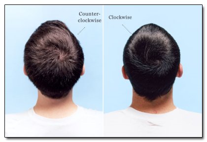
Lippa had gathered survey data from more than 50 short-haired men and photographed their pates (women were excluded because their hairstyles, even at the pride festival, were too long for simple determination; crewcuts are the ideal Rorschach, he explains). About 23 percent had counterclockwise hair whorls. In the general population, that figure is 8 percent.

Well, just how meaningful is this 23% discrepancy from the norm of 8%? Maybe it’s just randomness, right? Well, try the omitted calculations for yourself. This is an example of a “hypothesis test” in Statistics. The Null Hypothesis (H₀) says that there is no difference in the groups. The Alternative Hypothesis (H_A) says there is a statistically significant difference in the groups. In a hypothesis test, the essential question is this: What are the odds that a sample varies this much from the expected percentage (proportion) simply due to natural random variation? (For example, if you flip a coin 10 times, you usually get 5 heads. Sometimes, however, you might get 6. In fact, that should happen 26% of the time. Nothing to be alarmed about. However, the odds of getting 8 heads is only about 3%. If you do get 8 heads, that’s rare enough to indicate the coin might be rigged. Odds are you won’t do it again!)

So, for this hair test, we need to ask, “What are the odds of taking a sample of 50 guys and seeing that 23% having a counterclockwise whorl?” We should expect to get 8%, as per the broad population. If it’s very very rare to get 23%, then we might suspect there is a connection, and gay men do have different hair swirls than the broad population. In Statistics, we define “very very rare” as under 5%. In other words, if the odds that 23% of a sample of 50 have a counterclockwise whorl is under 5%, then it is statistically significant.

The calculations:

H₀: Gay men have no difference in their hair whorl orientation.
H_A: Gay men do have a difference in their hair whorl orientation.

First, take stock of the given information:

\(n = 50 \\\\ p = .08 \\\\ \hat{p}=.23\)

Next, you calculate the standard deviation of samples of this size.

\(SD(\hat{p})= \sqrt{\frac{(.08)(.92)}{50}}=.04\)

To determine how unlikely your sampling result was, you calculate how many standard deviations away from the expected proportion it was (Z-score).

\(Z(\hat{p})= \frac{\hat{p}-p_0}{SD(\hat{p})}=\frac{.23-.08}{.04}=3.75\)

\(p(Z \ge 3.75) = .000088 = 0\% \)

Conclusion: If the odds of having counterclockwise hair whorl is 8%, then the odds of having 23% of 50 random men exhibit this trait is unlikely. The odds of this happening by chance (random variations) is basically 0%. So, we reject the null hypothesis (H₀), and accept the alternative hypothesis (H_A)