Categories
Probability

Why Casinos Don’t Lose Money

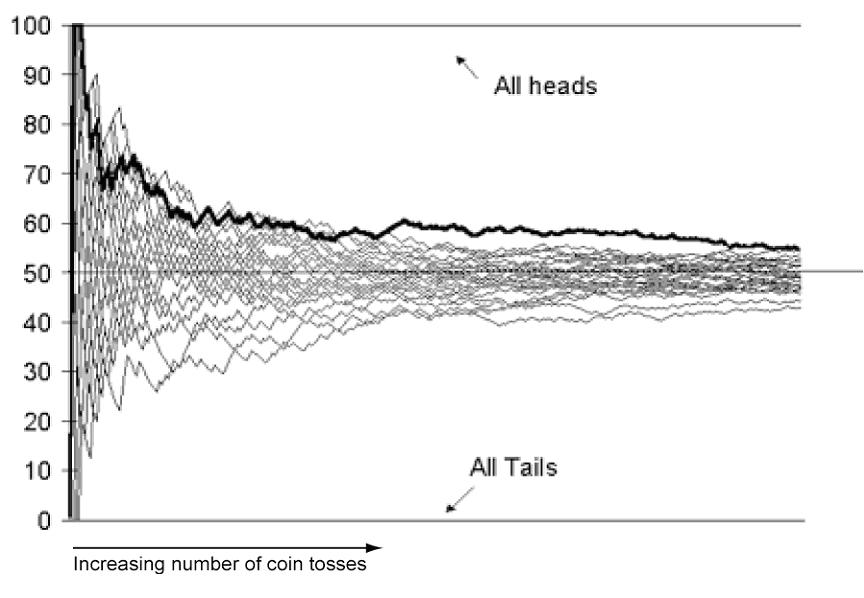
First, let’s illustrate the law of large numbers.  If you flipped a coin 10 times, you should expect to get 50% heads.  However, this may not happen.  You could get anything from 0 to 10 heads.  The most likely outcome is flipping 5 heads, and the odds of this outcome is 50%.  Variations from this become increasingly less probable.  For example, the odds of you flipping 4 or 6 heads is 26%, and the odds of you flipping 3 or 7 heads is 10%.  Now, let’s say you flipped a coin 100 times.  The odds of getting exactly 50% heads is still 50%.  But, do you think the odds of getting 60 heads is also 26%?  It’s actually only 2%.  It’s much easier to get 6 out of 10 heads, than it is to get 60 out of 100 heads.  What are the odds of flipping 600 heads out of 1000 flips?  It’s 0.00000001%.  With 1000 flips, you’re pretty much always going to get around 48%-52% heads.  Deviations beyond that range are very improbable.  So, in summary, the law of large numbers states that the more trials you have, the closer your actual outcome will be to the theoretical expected probability (In this case, the more coins you flip, the more you’ll start to approach actually getting 50% heads)

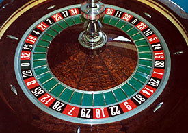
So, how does this tie into casinos?  Let’s take the roulette wheel as our example.  There are 37 total numbers.  18 reds, 18 blacks, and 1 green.  If you guess red or black correctly, you’ll get a 1:1 payout (ie: If you bet $1, you’ll get back $2, thereby winning $1).  If the wheel lands on green (0), both red and black lose.  This is where the casino gets it’s edge in this particular gamble.  Let’s calculate the expected value of a $1 bet on red.

\(E[X] = \frac{18}{37}(\$1)+\frac{18}{37}(-\$1)+\frac{1}{37}(\$-1) = -\$.03\)


What this means is you have an 18/37 chance of winning $1 (if it lands on red), and 18/37 chance of losing $1 (if it lands on black), and a 1/37 chance of losing $1 (if it lands on green)  The expected profit for playing this game is negative 2 cents.  Now, sometimes you’ll win, and sometimes you’ll lose, but if you play enough times, you’ll be averaging a loss of 23 cents per round.  This is where the law of large numbers comes into play.  As long as enough people are playing, the house will be averaging a profit of 2 cents for every dollar bet on that roulette table.

Question: What is the expected value of correctly guessing a specific number? There are 37 numbers, but the payout is 35:1 (You get paid $35 for each dollar you bet)  Based on this answer, is it smarter to try guessing the color or guessing the number?


Categories
Algebra 2

The Beatles meet Mathematics & Physics

About this sound Listen to the opening chord


Mathematics, Physics and A Hard Day’s Night

In this article we shall use mathematics and the physics of sound to unravel one ofthe mysteries of rock ’n’ roll – how did the Beatles play the opening chord of A Hard Day’s Night? The song may never sound the same to you again.


I just love this paper.  Professor Jason Brown sampled the famous opening chord of this song and (using Math) separated out all the distinct frequencies in the clip.  From this, he was able to determine each individual note that was played.  From there, he determined exactly what each member of the band played.  He even discovered a surprising element relating to George Martin’s 5th Beatle status.

Professor Brown took each frequency and converted it to a musical note on the Western scale.  Here is the function he used to do this:

\(f(x) = 12 log_2(\frac{x}{220})\)    (…where 220 hertz is the frequency for A natural.)

I thought I’d try his calculation myself, because it’s a good opportunity to use the change of base formula for logarithms.  If you look in the original white paper, the first frequency in the table is 110.34   Let’s plug this into the function:

\(f(110.34) = 12 log_2(\frac{110.34}{220}) = 12 log_2(.5015)\)

How do you evaluate the above expression?  There is no \(log_2()\) button on most calculators.  Well, here’s where the change of base formula for logs comes in:  \(log_b(x) = \frac{log_d(x)}{log_d(b)}\)   So, let’s choose \(log_{10}\) (since calculators do have this) and continue:

\(12 log_2(.5015)=12(\frac{log_{10}.5015}{log_{10}2}) = 12(-.9957) = -11.9466\)


In other words, 110.34hz is -11.9466 semi-tones below the note of A.  It should really be 12, but as Professor Brown noted, the Beatles’ instruments weren’t in perfect tune, so the values are not whole numbers!

So, which note is 12 semi-tones below A?  Actually, 12 semi-tones makes an octave, so the answer an A note.  Using this method, he determined every note that was played.  The rest of the paper describes how he deduced which groups of notes were played by which instrument/band member.  Fascinating.


Categories
Statistics

Does taking LSD prevent crime?

http://en.wikipedia.org/wiki/History_of_LSD

Dr. Leary began conducting experiments with psilocybin in 1960 on himself and a number of Harvard graduate students after trying hallucinogenic mushrooms used in Native American religious rituals while visiting Mexico. His group began conducting experiments on state prisoners, where they claimed a 90% success rate preventing repeat offenses. Later reexamination of Leary’s data reveals his results to be skewed, whether intentionally or not; the percent of men in the study who ended up back in prison later in life was approximately 2% lower than the usual rate.

Well, the question is this:  Was the drop from 92% down to 90% explained by random chance, or did the LSD really have a statistically significant impact on reducing the crime rate?  Since the text does not provide a sample size, I will just use n=100 to do the math.

The calculations:

H0:  LSD takers had no difference in their repeat offense rates.
HALSD takers did have a difference in their repeat offense rates.


First, take stock of the given information:

\(n = 100 \\\\ p = .92 \\\\ \hat{p}=.90\)


Next, you calculate the standard deviation of samples of this size.

\(SD(\hat{p})= \sqrt{\frac{(.92)(.08)}{100}}=.03\)


To determine how unlikely your sampling result was, you calculate how many standard deviations away from the expected proportion it was (Z-score).

\(Z(\hat{p})= \frac{\hat{p}-p_0}{SD(\hat{p})}=\frac{.90-.92}{.03}=-.67\)


Then, you calculate the odds of getting this Z-score via the normal cumulative distribution function.  (What are the odds of this happening randomly?)  If it’s under 5%, then you reject the null hypothesis, because it’s unlikely this variation can be attributed to random chance.  ie: Odds are, the hair is indeed different.

\(p(Z \le -.67) = .25 = 25\% \)


Conclusion:  If the odds of being a repeat offender is 92%, then the odds of having 90% (or less) repeat offenders in a random sample of 100 men is quite likely.  The math shows that the odds of this reduction simply happening by chance (random variations) is 25%.  This is large enough (over 5%), that we can not assume the LSD had any true effect on reducing crime rate.  ie:  The 2% reduction was probably due to chance.  So, we accept the null hypothesis (H0):  In a sample of 100 test subjects, the LSD had no effect if it only reduced the repeat offender rate to 90%.

 So, do you have the same lingering question that I did?  How large would the sample size have to be in order for the 2% drop to not be an accident? (Recall, I just made up n=100).  Well, some simple algebra should answer this for us:

First, let’s determine the Z-score at the 5th percentile:

\(invNorm(.05) = -1.64 \)


Let’s use that in the Z-score calculation to figure out what standard deviation we’d need

\(-1.64 = \frac{.90-.92}{SD}\)     (…SD = .012)


Backing this into the SD formula will help us solve for the sample size (n)
\(.012= \sqrt{\frac{(.92)(.08)}{n}}\)    (…n = 495)

So, if Timothy Leary showed a repeat offender drop of 2% with a sample size of 495, then we could say the LSD did have an effect.  Why?  Because that much of a drop only has a 5% chance of happening randomly.

Categories
Statistics

Average hours of sleep (normal distribution)

How Little Sleep Can You Get Away With?


Nice example of a real life phenomena closely modelling a Gaussian normal distribution.  The average hours of sleep on a weeknight (for males) was 6.9 hours with a standard deviation of 1.5 hours.  Using this data, let’s calculate what percentage of men get a good night’s sleep.  The diagram indicates 27%.

\(Z = \frac{8 – 6.9}{1.5} = .73\)


\(normalCDF(.73,99) = .23 = 23\%\)


Categories
Statistics

The Statistics of Gaydar

The Science of Gaydar

Lippa had gathered survey data from more than 50 short-haired men and photographed their pates (women were excluded because their hairstyles, even at the pride festival, were too long for simple determination; crewcuts are the ideal Rorschach, he explains). About 23 percent had counterclockwise hair whorls. In the general population, that figure is 8 percent.

Well, just how meaningful is this 23% discrepancy from the norm of 8%?  Maybe it’s just randomness, right?  Well, try the omitted calculations for yourself.  This is an example of a “hypothesis test” in Statistics.  The Null Hypothesis (H0) says that there is no difference in the groups.  The Alternative Hypothesis (HA) says there is a statistically significant difference in the groups.  In a hypothesis test, the essential question is this:  What are the odds that a sample varies this much from the expected percentage (proportion) simply due to natural random variation?  (For example, if you flip a coin 10 times, you usually get 5 heads.  Sometimes, however, you might get 6.  In fact, that should happen 26% of the time.  Nothing to be alarmed about.  However, the odds of getting 8 heads is only about 3%.  If you do get 8 heads, that’s rare enough to indicate the coin might be rigged.  Odds are you won’t do it again!)

So, for this hair test, we need to ask, “What are the odds of taking a sample of 50 guys and seeing that 23% having a counterclockwise whorl?”  We should expect to get 8%, as per the broad population.  If it’s very very rare to get 23%, then we might suspect there is a connection, and gay men do have different hair swirls than the broad population.  In Statistics, we define “very very rare” as under 5%.  In other words, if the odds that 23% of a sample of 50 have a counterclockwise whorl is under 5%, then it is statistically significant.


The calculations:

H0:  Gay men have no difference in their hair whorl orientation.
HA: Gay men do have a difference in their hair whorl orientation.


First, take stock of the given information:

\(n = 50 \\\\ p = .08 \\\\ \hat{p}=.23\)


Next, you calculate the standard deviation of samples of this size.

\(SD(\hat{p})= \sqrt{\frac{(.08)(.92)}{50}}=.04\)


To determine how unlikely your sampling result was, you calculate how many standard deviations away from the expected proportion it was (Z-score).

\(Z(\hat{p})= \frac{\hat{p}-p_0}{SD(\hat{p})}=\frac{.23-.08}{.04}=3.75\)


Then, you calculate the odds of getting this Z-score via the normal cumulative distribution function.  (What are the odds of this happening randomly?)  If it’s under 5%, then you reject the null hypothesis, because it’s unlikely this variation can be attributed to random chance.  ie: Odds are, the hair is indeed different.

\(p(Z \ge 3.75) = .000088 = 0\% \)


Conclusion:  If the odds of having counterclockwise hair whorl is 8%, then the odds of having 23% of 50 random men exhibit this trait is unlikely.  The odds of this happening by chance (random variations) is basically 0%.  So, we reject the null hypothesis (H0), and accept the alternative hypothesis (HA)


Categories
Algebra

Optimal Snowboard Length Formula

http://www.livestrong.com/article/87496-size-snowboards/

Evaluate your height. This is the best way to determine snowboard length. One typical formula used by professional snowboards is: rider height (in inches) x 2.54 x 0.88 = suggested snowboard length. This will help you to start narrowing down your snowboard choices.

When I saw this formula, I wondered what it meant.  Note that snowboards are measured in centimeter units.  Well, to convert inches to centimeters, you multiply by 2.54.  So, we’re converting height to centimeters and then taking 88% of that.  I have no idea where the 88% rule comes from.  The point being, the “formula” is just saying to get a snowboard that is 88% of your height.  This lines up with my mouth, and I am pretty sure I am well-proportioned.  So, maybe it’s just easier to say that a snowboard should come up to your mouth.

This is also an example of intentionally not simplifying an expression because you lose some inherent meaning (explicit unit conversion, etc).  Otherwise, the equation could be simplified to length = 2.235 * rider height (in inches)


Categories
Algorithms Computer Programming Statistics

How does Netflix predict which movies you’ll like best?

The simplest way to predict your rating for a movie is simply to average everyone else’s rating of the movie.  (ie:  They can just give you the 10 movies with the highest average rating)  Of course, it can get much more complex that than, especially when NFLX was giving away a million dollars to anyone who could improve their rating algorithm!  The real meta of this problem is to determine other people who are most like you, and then use their collective ratings on movies you haven’t seen yet.

Neighborhood-based model (k-NN): The general idea is “other people who rated X similarly to you… also liked Y”.  To predict if John will like “Toxic Avenger”, first you take each of John’s existing movie ratings, and for each one (eg: “Rocky”), find the people who rated both “Rocky” & “Toxic Avenger”.  You then compare the ratings given to both movies by these people, and calculate how correlated these 2 movies are.  If it’s a strong correlation between their ratings, then “Rocky” is a strong neighbor in predicting John’s rating for “Toxic Avenger”.  You’ll weigh in the average rating given (by “Rocky raters”) to “Toxic Avenger” highly.  You do this for all the movies that John has already rated, and find each one’s strongest neighbor(s), and calculated a predicted “Rocky” rating from each movie John has already rated.  You then calculate a weighted average of all these predictions to come up with your ultimate prediction for John’s rating of “Rocky”.  Lastly, if you do this for every movie in the entire database, you can determine a “Top 10 suggestions” list for John.


Here is some general reading on the contest:

The BellKor solution to the Netflix Prize

This Psychologist Might Outsmart the Math Brains Competing for the Netflix Prize

The Netflix Prize: 300 Days Later

The Greater Collaborative Filtering Groupthink: KNN


Categories
Set Theory

Links: Humor with Venn Diagrams

Le Grand Content

On the Origin of Venn Diagrams

http://thisisindexed.com/

Categories
Algorithms

How They Check if a Credit Card Is Valid

Before the era of ethernet, TCP/IP, and packet verification, electronic data was transmitted over telephone wires.  (Think back to the days of AOL & modems, and that screeching noise when you connected.)  A big problem with this method was the risk of external interference garbling your signal.  What if a bird flew into the phone wire?  Or if someone picked up the other line?   Or it started raining?  Any external interference could result in the  information being sent at that moment to be garbled.  So, if you were transmitting something like a credit card number, how would the receiver know that it wasn’t garbled?  (For example, what if a 3 was garbled into a 4?)   This was a problem solved at IBM back in the 1950s.  Of course, the same issues arise when human error is introduced.  (What if you are reading the credit card aloud over the phone, and the other person types in one of the digits incorrectly?)

For the rest of this post, I am merely introducing a lecture I attended called “Identification Numbers and Check Digit Schemes”, by Joe Kirtland.  Thanks to Joe for sharing his full PPT slides with me (link below).  It talks about the checkdigit systems used to validate credit cards, bar-codes, ISBN numbers, currency serial numbers, etc.  It’s a great real-world application of Algebra, Geometry, and algorithms.

Here is a very crude example that illustrates the concept:  Let’s say you want to transmit the number “34515”.  One validation algorithm requires that the sum of the individual digits be divisible by 10 (mod 10 = 0).  Currently, the sum of the digits is 18 (3+4+5+1+5=18)  So, to make the sum divisible by 10, you just tack on a 2 at the end , and transmit “345152”.  The receiver of the data is told to ignore that last number, which is called a check digit.  The receiver then adds the numbers up and sees if the sum is divisible by 10.  If even one number was changed, it won’t work*.  If the final number he gets doesn’t check out, something went wrong, and you need to resend.

*Question:  This method is not foolproof, can you think of some reasons why?

If this topic interests you, check out the following slides, where Joe explored check digits as they relate to UPC codes, ISBN numbers, credit cards, and serial numbers on various currency.

Click here to view Joe’s full PPT lecture


Categories
Algebra Puzzles

Algebra Puzzle: Married Men

In a room full of men, ¾ of them are married.
There are 6 more married men then unmarried.
How many married men are there?

Set up the equations…

Categories
Algebra Engineering

What’s more likely to break down: a car with 200 miles or 20,000 miles?

In manufacturing/engineering, there is a concept known as the bathtub curve.  In theory, something that is brand new (including a human being!) is more likely to have failures than something that is a little older and has worked out those early kinks.  Of course, once the product gets old, you’ll start having new reasons for failure (things wearing out).

I don’t have much to add on this topic, but I created this post this for two simple reasons:

  • First, it’s a nice example of a Cartesian graph that makes intuitive sense.  The aggregate blue curve indicates that new things can be lemons, then they work smoothly, and then they wear out and start breaking again.
  • Also, I think its a great example of an authentic real-life piecewise function.   As you can see, it has three very different sections.


Question: In terms of cars, do you think the blue curve above would be so symmetric?


Categories
Trigonometry

Projectiles: What’s the optimal angle at which to throw something? (to maximize distance)

Wow, a real life formula that uses the double angle trig. identities!  As you can see, the distance a projectile will travel is a function of:  velocity, gravity, and the launch angle.

First, a quick fraction review:  First, recall that \(\frac{1}{1000}\) is a lot smaller than \(\frac{1}{10}\).  Conversely, we can also agree that \(\frac{1}{100}\) is a lot smaller than \(\frac{99}{100}\).  ie: The bigger the denominator (and/or smaller the numerator), the lower the value of the (positive) fraction.

So, since v is in the numerator, the distance traveled (d) increases directly with velocity (in a big way, since it’s squared)  Next, since g is in the denominator, the distance traveled decreases as gravity increases.  (Makes sense, right?)


This is a graph of all Sin(x) values from 0 to 360.  The x-axis is divided into quadrants (0, 90, 180, 270, 360). Notice in the graph that Sin(x) rises from 0 to 1 as x rises from 0 to 90 degrees.  Then, it drops from 1 back to 0 as x rises from 90 to 180 degrees.

Refer back to the double angle \(Sin(2\theta)\) in the original formula up top.  So, as x rises from 0 to 45 degrees, 2x actually rises from 0 to 90, and the \(Sin(2\theta)\) value is increasing.  But, as x continues to rise from 45 to 90 degrees, 2x rises from 90 to 180, which means the \(Sin(2\theta)\) value is now decreasing.

So, what’s the ideal angle to throw something?  The one that maximizes the value of \(Sin(2\theta)\), since it’s a multiplier in the projectile formula.  Well, as you can see in the graph, Sin(90) = 1, the highest possible value for Sin(x).  So, the ideal launch degree is x = 45 (which puts 2x at 90).

So, now you know why the ideal angle in these video games is 45 degrees, and have an inkling of how programmers create classic games like these:

Categories
Probability

Quitting While You’re Ahead? Random Walks & Markov Chains

Question:  What if you walked up to a “fair” casino game (50/50 odds of winning) that pays even odds with $10,000, and said you would quit as soon as you’re up $1,000 ? (ie: You either walk out with $11,000 or keep playing until you lose everything)  What are the odds of you leaving the casino with a $1000 profit?

Markov Chain can virtually simulate many random walks of this experiment.  With a large enough sample size, you can get an accurate sense of the odds of walking out with $1,000.

The following code runs this simulation as many times as you want, and tells you how many times you got to $11,000.

#!/usr/local/bin/perl
#!/opt/bin/perl

use Getopt::Long;
use strict;

GetOptions("f:s", "debug", "v");

my $current_round = 0;
my $starting_amt = 10;
my $lost = 0;
my $won = 0;
my $current_amt;
my $x;
my $low_bound = 0;
my $high_bound = 11;

while ($current_round < 100) {
while ($current_amt > $low_bound && $current_amt < $high_bound) {

		#generate a 1 or 0
		$x = int(rand(1)+.5);

		#adjust to either +1 or -1
		if ($x == 0) {
			$x = -1;
		}

		# update total
		$current_amt -= $x;

		# print current total
		print "$current_amt ";

	}

	print "\n";

	#increment rounds won or lost...
	if ($current_amt == 0) {
		$lost++;
	} else {
		$won++;
	}

	#reset current amount for next round
	$current_amt = $starting_amt;

	$current_round++;
}

print "\nWon = $won\n";
print "Lost = $lost\n";

Answer:  Doing 100 rounds is a large enough sample size to get an accurate result.  On average,  you’ll walk out with $11,000 about 90% of the time you try this experiment.  Why is this still a bad idea?  In practice, gamblers rarely quit while they are ahead, and you still have that 10% odds of a total washout.  Recall, the expected value of this game is still break even.

Here is a sample output of 10 rounds:

Won = 9
Lost = 1

Categories
Logic

The Flawed Logic of the Low-Fat Movement

Remember truth tables?  If p, then q.  Inverse, Converse, Contrapositive, etc.  First, a quick review.  Take the true statement “If you paint, then you’re an artist”

  • Inverse: “If you don’t paint, then you’re not an artist.”
    (False.  What if you just sculpt?)
  • Converse:  “If you’re an artist, then you paint”
    (False.  What if you just sculpt?)
  • Contrapositive: “If you’re not an artist, then you don’t paint.”
    (Ok, true, because if you did paint, you’d be an artist)

The point is that only the contrapositive is logically equivalent to the original statement.

Now, take a look at the statement “If you eat fat, then you’ll increase the odds of cardiovascular disease.”  What’s the inverse?  “If you don’t eat fat, then you will not increase odds of cardiovascular disease.”  Well, as you know, the inverse is not logically equivalent to the original statement, and therefore can’t be assumed as true.  In this example, limiting fat can lead to eating more carbohydrates (while keeping protein intake constant), which may be linked to cardiovascular disease


Watch 29:15 to 31:23 for this example of the incorrectly assuming the inverse is also necessarily true.

By the way, this lecture was the subject of a recent NYMag article titled Is Sugar Toxic?