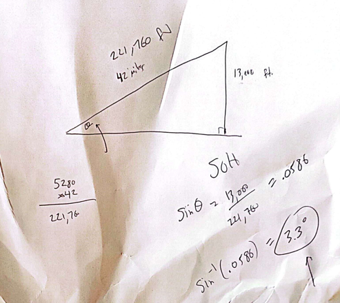
Mauna Kea on the Big Island of Hawaii is considered to be one of the hardest bicycle climbs in the world. It climbs 13,803 feet over 42 miles from sea level.
How steep is this climb?
Mauna Kea on the Big Island of Hawaii is considered to be one of the hardest bicycle climbs in the world. It climbs 13,803 feet over 42 miles from sea level.
How steep is this climb?

What if an investment returned 5%, 20%, and 50% over three years?
Year 1: $100 * .05 = $105
Year 2: $105 * .20 = $126
Year 3: $126 * .50 = $189
What was the annual return? Can you just average the percentages?
Let’s try it. The average of 5%, 20%, and 50% is 25%
Did you average 25% a year?
Year 1: $100 * .25 = $125
Year 2: $125 * .25 = $156.25
Year 3: $156.25 * .25 = $195.31
No, 25% for 3 years gets you a different amount!
You calculate the average annual return via the geometric mean (not the arithmetic mean)
\(\sqrt[3]{1.05 * 1.20 * 1.50} -1 = .236 \)
Your annual return was actually 23.6%
Year 1: $100 * .236 = $123.6
Year 2: $123.6 * .236 = $152.77
Year 3: $152.77 * .236 = $188.82 …

I noticed a for sale ad for a 1996 Mustang, and was struck by the $3500 price… ’94-‘04 Mustangs seem like a great bang for the buck: They are cheap, plentiful, have lots of parts available, and there’s lots of online DIY support. Perfect for a student or hobbyist on a budget.
I opened up 35 ads and noticed 19 were manual. I realized I was staring at a confidence interval problem!


If you have the only cell phone in the world, it’s pretty useless, since you can’t call anyone. If there are 2 cell phones, there is one possible connection. If there are 3 cell phones, you can make a total of 3 connections. 4 cell phones can have a total of 6 connections. 5 cell phones? 10 connections. 6 phones means 15 connections.
The more devices there are, the most connections you can make. The more connections there are, the more useful the whole network becomes. This is also called Metcalf’s Law.
Let’s look at the sequence of numbers generated above.
1, 3, 6, 10, 15, …
Can you see the pattern? The number of connections can be represented by \(\frac{n(n-1)}{2}\) where n is the number of nodes in the network. Notice that this is very similar to \(\frac{n^2}{2} = \frac{1}{2}n^2\). So, the number of total possible connections is proportional to the square of the number of nodes in the network.

The way this site works is that if you bid, you have to pay that amount, even if you lose. Bids are incremented by 1 cent. Let’s say an item sells for 10 cents. The guy who bid 1 cent still has to pay that, the guy who bid 2 cents still has to pay that, and so forth. So, what does the auction site actually earn for selling that item for 10 cents?
Notice that 1+2+3+4+5+6+7+8+9+10 can be added up by grouping numbers from the opposite ends: \((1+10) + (2+9) + (3+8) + (4+7) + (5+6)\) This is just \(11+11+11+11+11\) or 11*5 = 55. Note that when x = 10, and we ended up multiplying \(11*5\) for the series sum.
So, the general formula is:
1 + 2 + 3 + … + n = \(\displaystyle\sum\limits_{x=0}^n x = (n+1)\frac{n}{2} = \frac{n^2+n}{2} = \frac{n(n+1)}{2}\)
Pop Quiz! If the sunglasses in the photo end up selling for $6.96, how much does the website make? \(\frac{696*697}{2}\) = \(\frac{485112}{2}\) = \(242556\) = \(\$2,425.56\) !!
Which set is larger? The set of all positive integers {1,2,3,4,…} or the set of positive even integers {2,4,6,8,…} ?
In my dummy sports data below, you can see that the number of penalties is correlated most strongly to wins.

But, if you had hundreds of variables, how could you generate the cross product of every correlation possible, in order to find the variables with the highest correlation? One answer: Use the Stats program called “R” to create a correlation matrix! You can generate all sorts of visual outputs, as well. Penalties sticks out like a sore thumb now:


Disclaimer: Without stating a hypothesis up front, these finding is nothing more than “data snooping bias” (ie: curve fitting) The discovered association might simply be natural random variation, which would need to be verified with an out of sample test to have any validity at all.
To do this for yourself, here are the steps:
Enter the following commands in R:
(The lines with # are just comments, do not type them. Just paste the bold commands!
# Import data
> data1 <- read.csv(file.choose(), header=TRUE)
# Attach data to workspace
> attach(data1)
# Compute individual correlations
> cor(Penalties, Win)
# Scatterplot matrix all variables against each other
> pairs(data1)
# Generate a CORRELATION MATRIX !!
> cor(data1)
Here is how to generate the visual output:
> library()
…Scroll back up to the very first line of the popup window. Packages are probably in something like library ‘C:/Program Files/R/R-3.3.0/library’
Download and install “corrplot” Windows binaries package into the library path above.
Note: When you extract, you will see the folder heirarchy: corrplot_0.77/corrplot/….
Only copy the 2nd level folder “corrplot” into the library/ folder. (ie: Ignore the .077 top folder)
# import corrplot library
> library(“corrplot”)
# generate correlations matrix into M
# You now redirect the cor() function output we used above into a matrix called “M”
> M <- cor(data1)
# Plot the matrix using various methods
# Method can equal any of the following: circle, ellipse, number, color, pie
> corrplot(M, method = “circle”)
> corrplot(M, method = “ellipse”)
> corrplot(M, method = “number”)
> corrplot(M, method = “color”)
> corrplot(M, method = “pie”)
 Here is a question someone recently asked me: What’s the probability that two students taking a multiple choice test with 29 questions will get exactly the same wrong answers on 10 of the questions?

He returned for another round of Goldman’s grilling, which ended in the office of one of the high-frequency traders, another Russian, named Alexander Davidovich. A managing director, he had just two final questions for Serge, both designed to test his ability to solve problems.
The first: Is 3,599 a prime number?
Serge quickly saw there was something strange about 3,599: it was very close to 3,600. He jotted down the following equations: 3599 = (3600 – 1) = (602 – 12) = (60 – 1) (60 + 1) = 59 times 61. Not a prime number.
The problem wasn’t that difficult, but, as he put it, “it was harder to solve the problem when you are anticipated to solve it quickly.” It might have taken him as long as two minutes to finish. The second question the Goldman managing director asked him was more involved—and involving. He described for Serge a room, a rectangular box, and gave him its three dimensions. “He says there is a spider on the floor and gives me its coordinates. There is also a fly on the ceiling, and he gives me its coordinates as well. Then he asked the question: Calculate the shortest distance the spider can take to reach the fly.” The spider can’t fly or swing; it can only walk on surfaces. The shortest path between two points was a straight line, and so, Serge figured, it was a matter of unfolding the box, turning a three-dimensional object into a one-dimensional surface, then using the Pythagorean theorem to calculate the distances. It took him several minutes to work it all out; when he was done, Davidovich offered him a job at Goldman Sachs. His starting salary plus bonus came to $270,000.
The incidence of Alzheimer’s doubles every five years after the age of 65 until, by 85 years, nearly one in three adults is afflicted.
Are you wondering what percent are afflicted at age 65? Can you work backards from 33% being affected at age 85?
Let’s build up the equation. When something doubles, you multiply by 2. When it doubles a bunch of times, you will be multiplying by a bunch of 2’s… or simply \(2^n\) Since it is doubling every five years, you only want to multiply by 2 when the year hits a multiple of 5. So, change it to \(2^\frac{n}{5}\) You also need some sort of initial amount that is getting doubled in the first place. Our initial equation to represent the percent of people with Alzheimer’s at 65 is \(y=a(2^\frac{n}{5})\) Next, we use the given (n,y) pair to solve for that constant (a). At 85 years (ie: 20 years later), the percent is .33 So, plug it in. \(.33=a(2^\frac{20}{5})\) (Also, notice how the division by 5 comes into play? 20/5 = 4 doubles in that 20 years. ie: Doubles every 5 years) Solve and get a = .02 Plug that back into a, and you have \(y=.02(2^\frac{n}{5})\) Well, let’s answer the question. What percentage of people have Alzheimer’s at age 65 (n=0)? \(y = .02(2^\frac{0}{5}) = .02(2^0) = .02(1) = .02\) So, 2% of people at age 65. A quick calculation verifies this: 2, 4, 8, 16, 32 at ages 65, 70, 75, 80, 85, respectively.
In high school, you almost never see a “real” proof. You only see those Statement/Reason proofs in Geometry. These types of proofs never really show you what real math proofs are really like. So, here are 2 for you:
What an absolutely brilliant application of geometry!

Airplanes crashing! ATM machines stopping! Computers exploding!? What was the Y2K doomsday all about?
Most computer programs written prior to the mid 1990s used only 2 characters to keep track of the year. Back in the 1970s and 1980s, computing power was expensive, so it made sense not to waste 2 extra digits storing a bunch of redundant “19__” prefixes. The computer would simply store a 55 or 97, instead of 1955 or 1997.
The problem with Y2K was that any date calculation written this way would fail once the year rolled over to 2000. Why? Let’s look at a very simple example. Let’s say a computer program calculates how old you are in order to determine if you’re eligible for certain medical benefits. The code could look something like this:
birth_year = 29;
current_year = 95;
age = current_year – birth_year;
If (age >= 65) then medicare_eligible = TRUE;
Normally, this works fine. In the above example, the age = 95 – 29 = 66, and he can get medicare benefits. But, notice what happens when this same code runs in the year 2000 !
birth_year = 29;
current_year = 00;
age = current_year – birth_year;
If (age >= 65) then medicare_eligible = TRUE;
Now age = 00 – 29. That’s negative 29 years old. Clearly, -29 is not greater than 65. So, the computer thinks you’re not old enough to get medicare benefits! The logic goes haywire unless all the date codes are expanded to 4 digits. Once you do that, 2000 – 1929 = 71.
Apply this simple calculation error to anything that needed to compare dates, or determine how old something is, or how much time has passed. This is why people were expecting a computing catastrophe when the date rolled over.

I was replacing the power steering fluid in my car when I stumbled upon some exponential decay math. First, some background: There is no drain plug on a power steering system. You need to siphon out fluid from the reservoir and replace it with new fluid. This new fluid then mixes into the rest of the system to create a slightly cleaner mixture. This idea is that if you repeat this a few times, you’ll replace most of the old fluid with new fluid.
So, as you can see, there exists some sort of formula that can determine exactly how many times you need to extract and replace to reach X% replacement.
My car’s entire power steering system holds about 1 liter, and the reservoir itself holds .4 liters of that. So, 40% of the steering fluid is replaced each time I drain and refill the reservoir, and 60% of the old fluid remains elsewhere in the system. I can do this repeatedly, each time replacing 40% of the “mixed” fluid with brand new fluid.
Let p = Percentage of the system replaced each time you empty the reservoir.
Let n = number of times you empty/fill the reservoir (“flush”)
Let FD = Percentage of dirty fluid in the system.
Let FN = Percentage of new fluid in the system.
If p = percentage of new fluid introduced by a flush, then (1-p) is percentage of old fluid remaining. (eg: if \(p = .40, then (1-.40) = .60)\)
\(FD_0 = 1\) (initial proportion that is dirty)
\(FD_1 = (1-p)\)
\(FD_2 = (FD_1)(1-p) = (1-p)(1-p)\)
\(FD_3 = (FD_2)(1-p) = (1-p)(1-p)(1-p)\)
…
\(FD_n = (FD_{n-1})(1-p) = (1-p)^n\)
\(FD = (1-p)^n\)
\(FN = 1 – FD\)
For my car, p=.40 so \(FD = (1-.40)^n\)
How many times do I need to empty and fill the reservoir to get to 80% clean?
Just set \(FN = .8\) and solve for n:
\(.80 = 1- (1-.40)^n\)
\(.80 = 1- (.60)^n\)
\(.6^n = .2\)
\(log(.6)^n = log(.2)\)
\(n*log(.6) = log(.2)\)
\(n = \frac{log(.2)}{log(.6)}\)
\(n = 3.15\)
With a reservoir that holds 40% of capacity, I need to empty and replace it about 3 times to get 80% of the old fluid replaced.
You can also use the formula to figure out what percentage of the system contains old vs. new fluid, based on the number of flushes you’ve done. For this, you just plug in n and calculate \(FD\) eg: If you’ve done 5 flushes, \(FD = (1-.4)^5 = .08\) So, after 7 refills, 8% is dirty, and 92% is new.


In a nutshell, the sin() and cos() terms are periodic curves, and the weighting of the various coefficients is what allows proper regression fits. Let’s take a closer look at the formula, and try to make sense of it.
For example, as t goes from 0 to 52, \(\frac{t}{52}\) goes from 0 to 1, \(2\pi * \frac{t}{52}\) goes from 0 and 360. (and then it repeats since sin repeats in multiples of \(2\pi\) and therefore \(sin(2\pi * \frac{t}{52})\) goes from sin(0) to sin(360) which is a full periodic cycle of this function. Note the same logic applies to the cos() term in the formula.
The picture says it all.

Further Reading: Automated Detection of Influenza Epidemics with Hidden Markov Models

The essence of fractal geometry lies in recursive iteration. What’s that? It’s just a self-referring loop. Let’s start with a simple equation: \(f(x)=2x+1\)
Let x=0 and plug it in, and you’ll get a 1:
\(f(0)=2(0)+1=1\)
(Now, take that 1 and plug it back into the same equation)
\(f(1)=2(1)+1=2\) (Then, take this 2 and do the same thing)
\(f(2)=2(2)+1=5\)
\(f(5)=2(5)+1=11\)
\(f(11)=2(11)+1=23\)
And so forth. You can keep doing this forever, and notice how this list of results (0,1,2,5,11,…) will tend towards infinity (This isn’t always the case)
The mother of all fractals, the Mandelbrot Set is defined by this deceptively simple equation: \(f(z)=z^2+c\) where c is some fixed constant. If you do the same procedure above, you’ll get a series of numbers. eg: Let c=5, and let’s start with z=0:
\(f(0)=0^2+5=5\)
\(f(5)=5^2+5=30\)
\(f(30)=30^2+5=905\)
At IBM, Benoit Mandelbrot used a complex number (a+bi) for that constant. For example, let’s use \(c=1+i\), as he did in his 1980 Scientific American article introducing fractals:
\(f(0)=0^2+(1+i)=1+i\)
\(f(1+i)=(1+i)^2+(1+i)=(1+i)(1+i)+(1+i)=(1+2i+i^2)+(1+i)=2i+(1+i)=1+3i\)
\(f(1+3i)=(1+3i)^2+(1+i)=(1+3i)(1+3i)+(1+i)=(1+6i+9i^2)+(1+i)=6i-8+(1+i)=-7+7i\)
…and so on. For the Mandelbrot set, the calculation is iterated until it’s clear whether the result is tending towards 0 or infinity. Based on this result, for every complex number, you plot a point on the complex plane either black or white. (Or, it is colored based on how fast it tends towards infinity.) For example, 1+i tends towards infinity when plugged into this equation, so a black point is plotted for 1+i on the complex plane. This process was then repeated for every complex number, and was only possible because of the advent of modern computers. Every single complex number gets a point (eg: .234234234 + .324325423i) The result is the deeply infinite, self-referential image you see above. The image is much more complex than it appears. For example, if you zoom in to a certain section, you will see the entire image repeat within itself, and then repeat within that zoom! I can’t do it justice here, so if you want to learn how this Math models real life phenomena & situations, these 2 videos are a great primer for a layman:

So, I was talking to a friend about how pullups need more rest time between sets than other exercises:
Pullups need significant recovery time to not have logarithmic decay in the number of reps you can do.
I suggested waiting about 3 minutes between sets. Of course, the next time I did them, I wanted to see just how logarithmic the decay is. I plugged the numbers into Excel and did a log regression. Wow, I wasn’t kidding, look at that correlation coefficient !!


The lens in this photo has a focal length of 50mm. In general, the higher the focal length, the more zoom you’ll have. For example, a wide angle lens is between 9mm-24mm, where a zoom/telephoto lens can be 150-400m. However, let’s focus on the list of numbers on the bottom edge of the lens: 1.4, 2.8, 4, 5.6, 8, 11, 16. At first glance, this is a bizarre sequence of random numbers. These numbers allow you to choose the f/stop, which is the ratio between the diameter of the lens opening (aperture) and the focal length of the lens. For example, for an f-stop of 2 (written f/2.0) the diameter would be 25mm while the focal length is 50mm, because 25mm divides into 50mm two times. Hence, the general equation is: \(f/stop = \frac{focal\ length}{diameter}\) Note that when the f/stop is low, it means the aperture is large. (FYI, the point of a large aperture is to let in a ton of light to improve picture quality).

Next, let’s play around with some numbers and see where this leads us. The simplest example would be to consider an f/stop ratio of 1 (written f/1.0) on a 50mm lens: This would mean the diameter of the lens opening (aperture) is 50mm, making the radius equal to 25mm. Remember the old circle formulas from middle school? Well, knowing the radius, we can calculate the actual area of the lens opening at f/1.0.

\(Area = \pi r^2\)
\(Circumference = 2 \pi r = \pi d\)
\(A = \pi r^2 = \pi (25)^2 = 1963.5\)
Ok, so let’s try an f/stop that is actually on the lens (f/1.4):
\(1.4 = \frac{50}{diameter}\) … (so d = 35.7 and r = 17.86)
\(A = \pi r^2 = \pi (17.86)^2 = 1001.8\)
An f/1.4 lens has an aperture area of about 1000. Do you see any relationship between the area for f/1.0 vs. f/1.4? If not, I plugged in the rest of the f/stop numbers printed on the lens into a spreadsheet. What do you notice about the area of the circle for each subsequent f/stop?

In fact, the f/stop numbers that initially seemed so random actually do have a very precise relationship to each other. The area of the circle is being approximately halved for each of these f/stops. Conversely, for each f/stop you drop down, you are doubling the area of the lens aperture (effectively doubling the amount of light that the lens will let in!) Compare f/16 to f/1.4. They are 7 stops apart, meaning the amount of light doubles seven times. That means an f/1.4 lens allows 27 = 128 times as much light as the f/16 lens!! That makes a huge impact on the kind of pictures you can take when lighting is not optimal (indoors, night, etc). Most pocket cameras are about f/4. Even an f/2 lens will allow 4x as much light in (2 stops down)

RE: Birthday Dinner
Yes, life does go by fast. Strangely, the older you get, the faster it goes. I do not know why this is.
Ever get an email like this? Well, as your age varies, the percentage of your life that a single calendar year represents also varies. As you get older, a year is a smaller percentage of your overall life. In other words, 1 year represents 50% of a 2 year old’s life. However, it is only 2% of a 50 year old’s life. So, perhaps that is why each year seems to go by faster.
Want to see the percentage for every age from 0 to 80? Let’s make a formula and graph it. The percentage of your life that a single year represents is just a function of your age: \(f(age) = \frac{1}{age}\) If you graph this on a spreadsheet, you’ll get the following:

How would you interpret this graph? You’ll notice that once you pass the inflection point, the percentage seems to flatten out. So, at what point can a person legitimately start saying “Wow, this year really flew by?” Based on the graph, teenagers might feel this almost as much as middle aged people.
Lastly, do you notice how scaling of the y-axis makes the difference between age 15 and 50 look trivial? In order to properly display percentage changes, I will scale the y-axis logarithmically. Here is the result:

With this scaling, you can see a year in the life of a teenager (~6%) is quite different than a year in the life of someone in their 50s (~2%)
The Wallaby That Roared Across the Wine Industry
By the end of 2001, 225,000 cases of Yellow Tail had been sold to retailers. In 2002, 1.2 million cases were sold. The figure climbed to 4.2 million in 2003 — including a million in October alone — and to 6.5 million in 2004. And, last year, sales surpassed 7.5 million — all for a wine that no one had heard of just five years earlier.
Prima facie, it looks like exponential growth. But, in the real world, nothing ever grows exponentially in perpetuity (except college tuition, it seems) I looked up sales figures for other years online. Let’s plot these numbers in a spreadsheet, and see how they look. As you can see the growth started to flatten out after a few years.  I actually couldn’t find the sales data for 2008, so this calls for a statistical regression (fancy words for “line of best fit”). A linear regression only yielded r=.88, while a 2nd degree polynomial (quadratic) regression gave an r = .96. This regression equation is \(f(x) = -.13x^2 + 513x – 515887\)
Do you notice the negative leading coefficient of the x2 term? Remember how this makes the parabola “frown”? Well, this “inverted parabola” shape clearly reflects the flattening of the sales growth. 
By just looking at the trendline,what’s your estimate for the number of cases sold in 2008? Or, plug 2008 into the equation to get the exact coordinates on the red trendline: \(f(2008) = -.13(2008)^2 + 513(2008) – 515887 \)
